Computing Bounds for Clamped Means

Sometimes, the settings for private algorithms can inadvertently reveal private information.

Consider computing average energy use for a rural zip code. The largest energy consumer here may not consume very much energy, and the noise needed for differential privacy would not be very high, say \(\pm1,000\)kWh.

Imagine, then, that a wealthy environmentalist moves into the neighborhood. This person’s house, while proclaimed an efficiency engineering masterpiece, happens to consume much more electricity than expected, much more than neighboring houses (perhaps our environmentalist couldn’t resist running a bitcoin rig in the basement).

Now, because of the increased range of the dataset, obscuring this zip code’s total energy use requires more noise; instead of \(\pm1,000\) kWh it would be \(\pm10,000\) kWh. If we use the exact upper and lower bound of the dataset to scale DP noise, the confidence interval published alongside it would reveal our environmentalist’s embarassingly high energy usage almost exactly. Oops!

The solution to this problem is to privately compute the required scale of noise before computing the private mean. In this notebook, we employ a method that focuses on ease of implementation and high accuracy that does not minimize the privacy budget consumed.

By the end, we’ll have made sure not to have inadvertently publicly shamed our high-profile environmentalist.

# Preamble: imports and figure settings

from eeprivacy import (
  PrivateClampedMean,
  PrivateQuantile,
  laplace_mechanism,
)

import matplotlib.pyplot as plt
import numpy as np
import pandas as pd
import matplotlib as mpl
from scipy import stats

np.random.seed(1234) # Fix seed for deterministic documentation

mpl.style.use("seaborn-white")

MD = 28
LG = 36
plt.rcParams.update({
    "figure.figsize": [25, 7],
    "legend.fontsize": MD,
    "axes.labelsize": LG,
    "axes.titlesize": LG,
    "xtick.labelsize": LG,
    "ytick.labelsize": LG,
})

Dataset

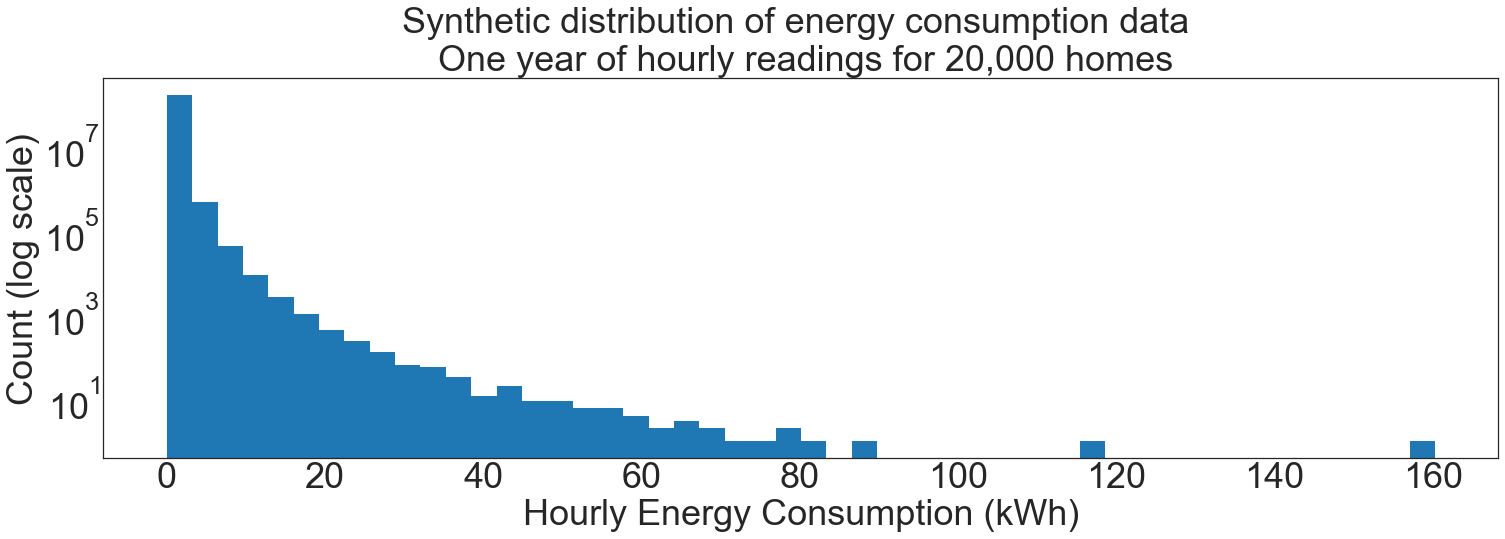
For this example, we consider a dataset of one year of hourly energy consumption readings from 20,000 homes. In total, there are 20,000 * 365 * 24 = 175,200,000 data points, with each home contributing 8,760 each.

From experience, we know this sort of dataset follows a power law distribution.

N = 20000
hourly_consumption_kwh = np.random.pareto(4, N*365*24)

fig, ax = plt.subplots()
ax.hist(hourly_consumption_kwh, bins=50)
ax.set_yscale("log")
plt.title(f"Synthetic distribution of energy consumption data \n One year of hourly readings for {N:,} homes")
plt.xlabel("Hourly Energy Consumption (kWh)")
plt.ylabel("Count (log scale)")
plt.show()

Background Theory

To compute a differentially private mean, noise is drawn from the Laplace distribution at \(b=\Delta/\epsilon\) where \(b\) is the scale of the Laplace distribution, \(\Delta\) is the sensitivity, and \(\epsilon\) is the privacy parameter.

The unknown parameter in this case is the sensitivity \(\Delta\). For private means, the sensitivity is:

\[\Delta = \frac{B - A}{N}\]

Where \(B\) is largest value in the dataset, \(A\) is the smallest, and \(N\) is the number of elements in the dataset. Intuitively, the sensitivity is the maximum amount that any single element in the dataset can affect the computed mean.

For datasets where the range of data is known up front, the values of \(A\) and \(B\) are known exactly.

However, for datasets where the range of data can vary considerably, the values of \(A\) and \(B\) must be computed with a private query to avoid leaking information about the largest and smallest values in the dataset.

Approach to Privately Finding Bounds

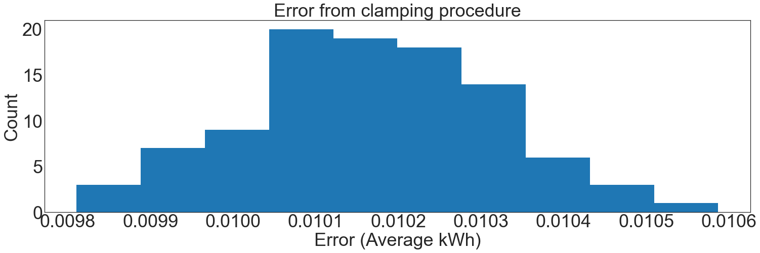
First, we define a criteria for a good choice of upper bound. The eventual use for building science requires private means to be accurate within +/-0.1 kWh. Since the error term for the clamping procedure is difficult to derive exactly, we will target error from the clamping procedure as small enough to be neglible compared to the required accuracy. Therefore, we target +/-0.01 kWh.

To find the upper bound for this level of accuracy, we simulate clamping random samples from our synthetic dataset. We find that a clamping cutoff that includes 99% of all consumption values reaches this target error:

def simulate_clamping_error(number_of_sites, cutoff):
  NS = number_of_sites
  HY = 8760 # hours per year
  trials = []
  for t in range(100):
      sample = np.random.choice(hourly_consumption_kwh, NS * HY)
      true_mean = np.mean(sample)
      clipped_mean = np.mean(np.clip(sample, 0, cutoff))
      trials.append(true_mean - clipped_mean)

  plt.hist(trials)
  plt.title("Error from clamping procedure")
  plt.xlabel("Error (Average kWh)")
  plt.ylabel("Count")
  plt.show()


cutoff = 2.2
simulate_clamping_error(number_of_sites=200, cutoff=cutoff)

percent_included = np.sum(hourly_consumption_kwh <= cutoff) / len(hourly_consumption_kwh)
print(f"The cutoff includes {percent_included:.2%} percent of consumption readings")

The cutoff includes 99.05% percent of consumption readings

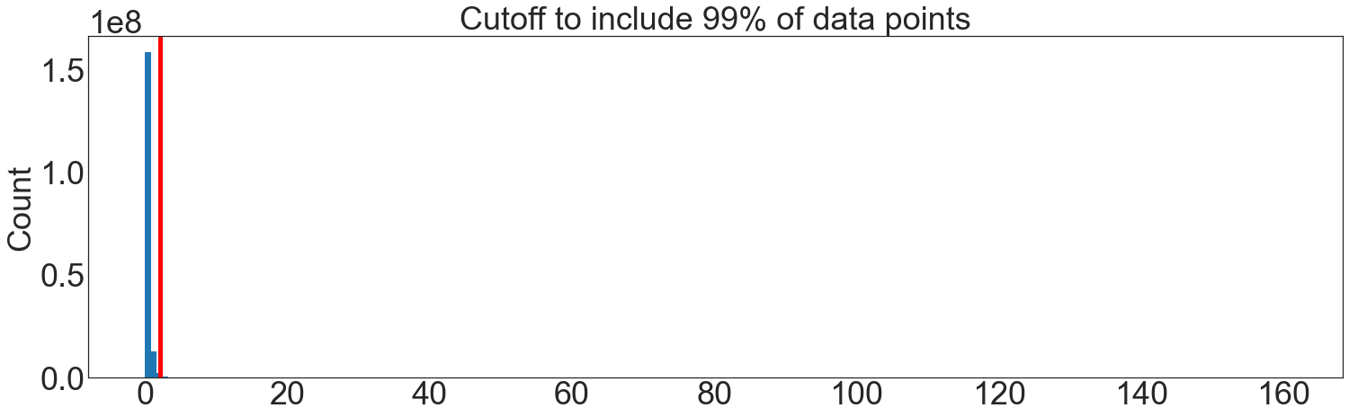
If we were able to query for the distribution of data exactly, we would ask for the 99th percentile directly.

cutoff = np.quantile(hourly_consumption_kwh, 0.99)

print(f"The 99% cutoff is {cutoff:.1f} kWh")

plt.hist(hourly_consumption_kwh, bins=200)
plt.axvline(cutoff, color="r", linewidth=5)
plt.title("Cutoff to include 99% of data points")
plt.ylabel("Count")
plt.show()

fig, ax = plt.subplots()
ax.hist(hourly_consumption_kwh, bins=50)
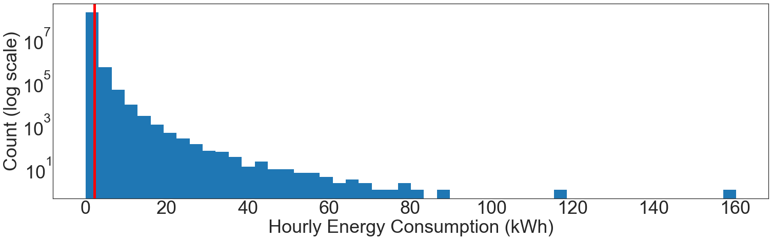
ax.set_yscale("log")
plt.axvline(cutoff, color="r", linewidth=5)
plt.xlabel("Hourly Energy Consumption (kWh)")
plt.ylabel("Count (log scale)")
plt.show()

The 99% cutoff is 2.2 kWh

However, this query must be done privately to avoid leaking information. Fortunately, there is a mechanism that can be used to answer this question directly: eeprivacy.private_quantile.

Private Quantiles

Under the hood, eeprivacy.PrivateQuantile uses a “private noisy max” mechanism to score a set of possible outputs. In this case, the outputs are choices for quantiles.

The following code finds the 99th percentile:

result = PrivateQuantile(
  options=np.linspace(0, 5, num=200),
  max_individual_contribution=8760
).execute(
  values=hourly_consumption_kwh,
  quantile=0.99,
  epsilon=0.1,
)

print(f"Private 99th percentile is {result:.2f} kWh")

Private 99th percentile is 2.24 kWh

Private Quantile Accuracy

An appropriate choice of \(\epsilon\) is required for private_quantile. Too high, and too much privacy budget is spent. Too low, and a poor clipping bound risks introducing error to all further analyses.

For this demonstration, we show that a choice of \(\epsilon\)=0.1 provides a distribution of results that are within acceptable boundaries based on the earlier accuracy simulation.

# Unroll the implementation of `private_quantile` for performance reasons:
# computing `scores` is quite heavy and only needs to be done once.

values = hourly_consumption_kwh
options = np.linspace(0, 5, num=200)
quantile = 0.99
epsilon = 0.1
sensitivity=8760

N = len(values)

def score(values, option):
    count = np.sum(values < option)
    return -np.abs(count - N * quantile)

scores = [score(values, option) for option in options]

trials = []

for t in range(100):
  noisy_scores = laplace_mechanism(
      values=scores, epsilon=epsilon, sensitivity=sensitivity
  )
  max_idx = np.argmax(noisy_scores)
  result = options[max_idx]
  trials.append(result)

plt.hist(trials)
plt.title(f"Distribution of private 99th percentile at ε={epsilon}")
plt.xlabel("99th percentile result")
plt.ylabel("Count")
plt.show()

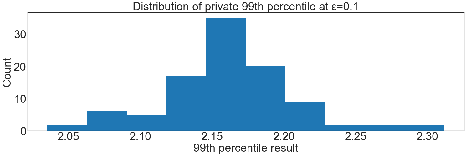
This choice of privacy parameter is not optimal; it could be further reduced and still meet accuracy needs. In the work that this demo was based on, there was enough privacy budget allocated that \(\epsilon\)=0.1 did not hamper further analysis.

Results

In our example, the final computed clamping bound was 2.16 kWh. There was some error introduced in choosing the clamping boundaries with the private quantile mechanism.

To get a feel for this error, we use our original accuracy simulation for the upper and lower bounds of results from the private quantile function, comparing it to an exact mean computation:

def simulate_clamping_error(number_of_sites, cutoff):
  NS = number_of_sites
  HY = 8760 # hours per year
  trials = []
  for t in range(100):
      sample = np.random.choice(hourly_consumption_kwh, NS * HY)
      true_mean = np.mean(sample)
      clipped_mean = np.mean(np.clip(sample, 0, cutoff))
      trials.append(true_mean - clipped_mean)

  plt.hist(trials)
  plt.title(f"Error from clamping procedure (cutoff={cutoff})")
  plt.xlabel("Error (Average kWh)")
  plt.ylabel("Count")
  plt.show()

simulate_clamping_error(number_of_sites=200, cutoff=2.05)
simulate_clamping_error(number_of_sites=200, cutoff=2.30)

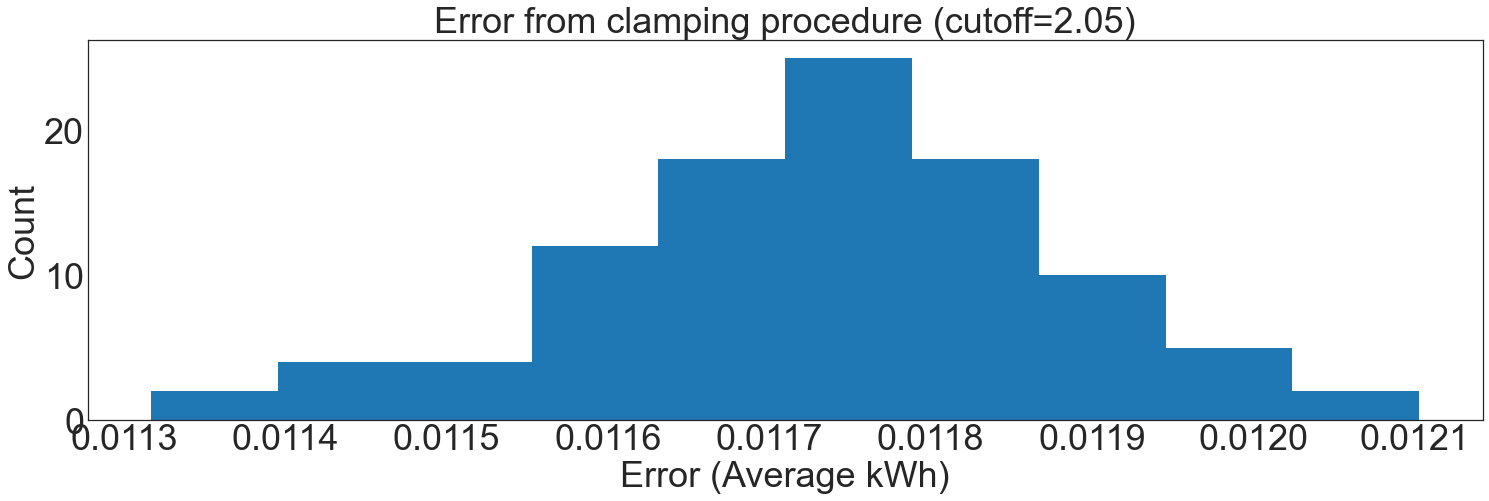
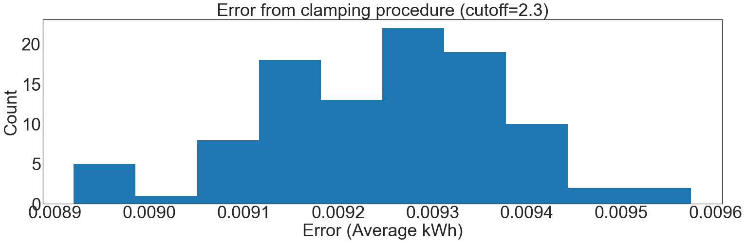
The resulting error is within \(\pm0.01\) kWh in all cases. This is well-suited for the statistics that will be prepared with these data, which can tolerate at least +/- 0.1 kWh of error, an order of magnitude more.