Stochastically Testing Privacy Mechanisms

How do you validate that a differential privacy implementation actually works?

One approach that can build confidence that the differential privacy property holds for an implementation is stochastic testing: run many iterations of the algorithm against neighboring databases and check that for any output, the expected probability is bounded by \(\epsilon\).

# Preamble: imports and figure settings

from eeprivacy import PrivateClampedMean

import matplotlib.pyplot as plt
import numpy as np
import pandas as pd
import matplotlib as mpl
from scipy import stats

np.random.seed(1234) # Fix seed for deterministic documentation

mpl.style.use("seaborn-white")

MD = 20
LG = 24
plt.rcParams.update({
    "figure.figsize": [25, 7],
    "legend.fontsize": MD,
    "axes.labelsize": LG,
    "axes.titlesize": LG,
    "xtick.labelsize": LG,
    "ytick.labelsize": LG,
})

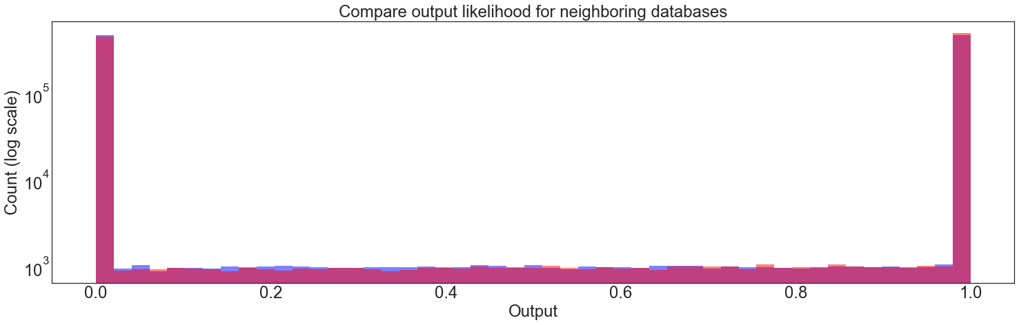
In the test below, we run a PrivateClampedMean for a large number of trials for two different databases: one with a single element 0 and one with a single element 1.

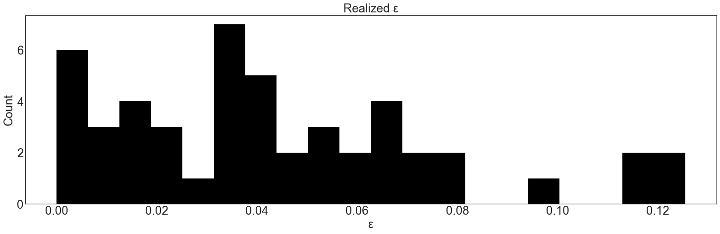
Then, we bin the results and compute the “realized \(\epsilon\)” for each bin. By chance, sometimes this will slightly exceed the \(\epsilon\) value. The test fails if the realized \(\epsilon\) greatly exceeds the desired \(\epsilon\) for any of the bins.

private_mean = PrivateClampedMean(lower_bound=0, upper_bound=1)

T = 1000000
A = [private_mean.execute(values=[], epsilon=0.1) for t in range(T)]
B = [private_mean.execute(values=[1], epsilon=0.1) for t in range(T)]

L = 0
U = 1

A = np.clip(A, L, U)
B = np.clip(B, L, U)

bins = np.linspace(L, U, num=50)

fig, ax = plt.subplots()
ax.set_yscale("log")

plt.hist(A, color='b', alpha=0.5, bins=bins)
plt.hist(B, color='r', alpha=0.5, bins=bins)
plt.title("Compare output likelihood for neighboring databases")
plt.xlabel("Output")
plt.ylabel("Count (log scale)")
plt.show()

A, bin_edges = np.histogram(A, bins=bins)
B, bin_edges = np.histogram(B, bins=bins)

realized_epsilon = np.abs(np.log(A / B))

plt.hist(realized_epsilon, color="k", bins=20)
plt.title("Realized ε")
plt.xlabel("ε")
plt.ylabel("Count")
plt.show()